how to construct individual patient data that generates SEER relative survival curves
The National Cancer Institute’s (NCI’s) Surveillance, Epidemiology, and End Results (SEER) cancer statistics database provides three different types of summary survival curves:
- Observed survival: The proportion of patients who have not died of any cause by time \(t\) since diagnosis.
- Expected survival: The expected proportion of patients who have not died of any cause by time \(t\) since diagnosis, based on the all-cause mortality of a comparable group of people with respect to age, sex, race, calendar year, etc.
- Relative survival: The proportion of patients who have not died of cancer by time \(t\) since diagnosis, computed as the ratio of observed to expected survival.
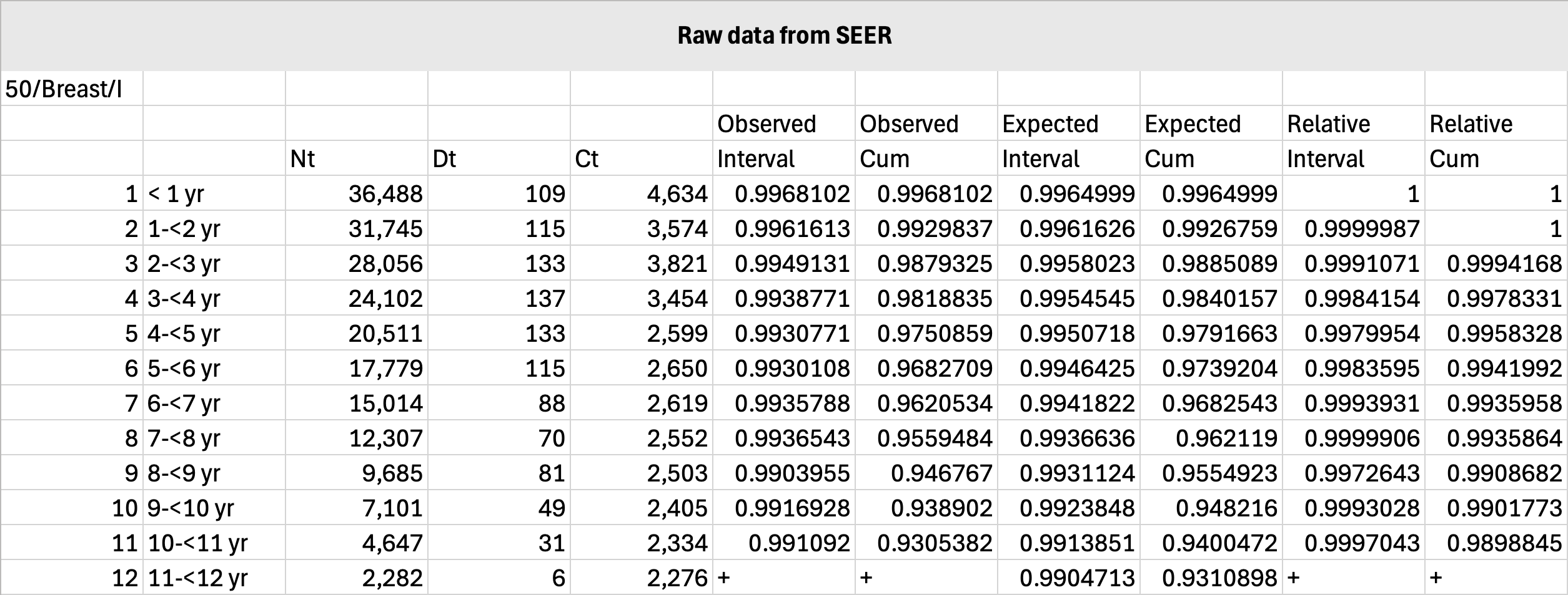
Survival curve fitting requires individual patient data (IPD) as an input. IPD can be constructed from counts of patients, deaths, and censored cases, which the SEER database provides in the following format:
- \(N(t)\): The number of patients still under observation by time \(t\) since diagnosis.
- \(D(t)\): The number of any-cause deaths by time \(t\) since diagnosis.
- \(C(t)\): The number of patients lost to follow-up by time \(t\) since diagnosis.
Constructing IPD for observed survival is straightforward since \(N(t)\), \(D(t)\), \(C(t)\) can be used directly. Constructing IPD for relative survival is not straightforward because \(N(t)\), \(D(t)\), \(C(t)\) need to be adjusted to reflect cancer deaths only. This tutorial will demonstrate how to do so.
MASSIVE DISCLAIMER!!! I am in no way claiming that this is the right thing to do. To be totally correct, i.e., abiding by the definition of relative survival, one should generate IPD for observed and expected survival, fit the curves separately, then compute relative survival as their ratio. The below method is simply a hack to quickly generate relative survival curves. It will not preserve the relationship between observed, expected, and relative survival after curve fitting. Proceed with caution.
Let \(R(t)\) denote the interval (NOT cumulative) relative survival probabilities. This tells us the proportion of patients from time \(t-1\) who are still alive at time \(t\) for \(t>0\), with \(R(0)=1\).
The number of patients under observation does not change, so:
\[N^\ast(t)=N(t).\]The number of censored cases should be augmented with the number of non-cancer deaths, since their death from other causes effectively renders their time of cancer death unobservable:
\[C^\ast(t)=C(t)+D(t)-D^\ast(t).\]Now since we are reframing cancer survival as observed survival, we have the following relationship (using the actuarial method):
\[R(t)=1-\frac{D^\ast(t)}{N^\ast(t)-\tfrac{1}{2}C^\ast(t)}.\]Solving for \(D^\ast(t)\) yields:
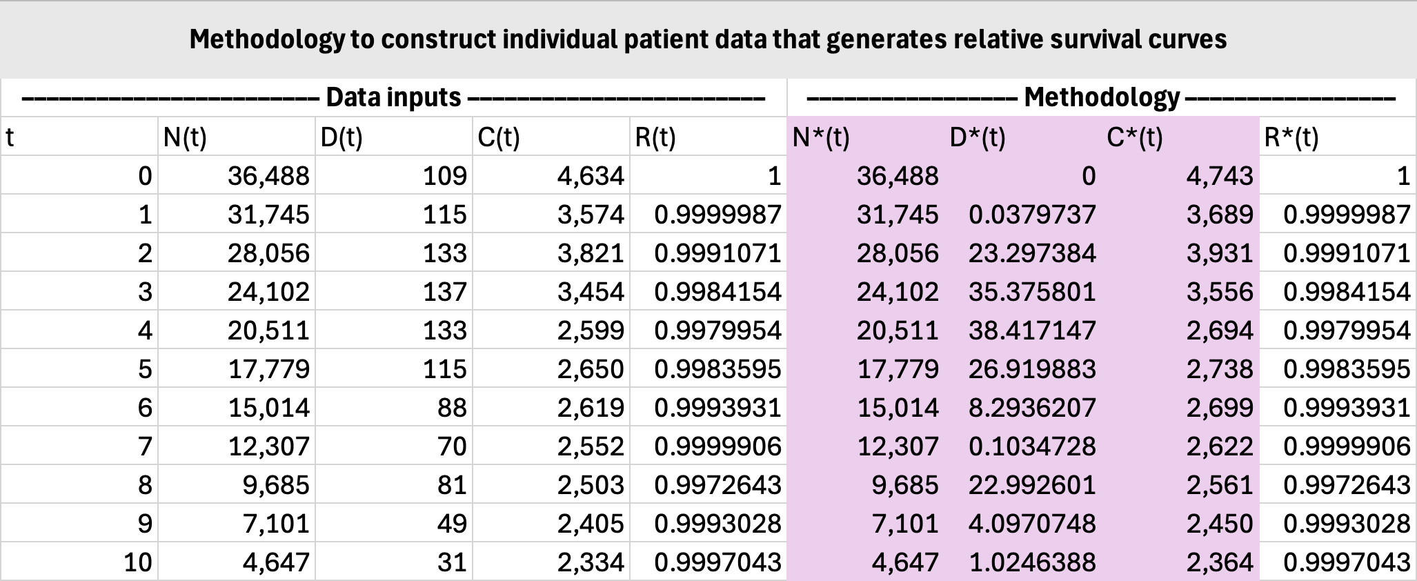
\[D^\ast(t)=\frac{\big(2N(t)-C(t)-D(t)\big)\big(1-R(t)\big)}{1+R(t)}.\]The remaining step is to construct the IPD itself. The precise methodology is detailed elsewhere, e.g., Hoyle et al. (2011).
Below is a sample calculation using SEER data for stage I breast cancer diagnosed at age 50 years: